Analyzing 530,000 Black Friday transactions data using MSSQL and PowerBI
This paper analyzes 530,000 Black Friday transactions data using MS SQL. The analysis reveals a consumption distribution tending towards the 70/30 rule, with 30% of individuals accounting for nearly 70% of the consumption. The most powerful spending demographic is the group consisting of males aged 26 to 35 who are unmarried. Finally, a PowerBI dashboard is constructed to visualize the results.

The data

The dataset blackfriday is from Kaggle. It consists of 9 columns:
1. User_ID: Each user may make multiple purchases, so it is not a unique value.
2. Product_ID: Product identification number.
3. Gender: Categorical variable indicating gender.
4. Age
5. Occupation: Occupation of the user, with 20 categories. However, the specific meanings behind these categories are not provided.
6. City_Category: Categorical variable indicating the city category, with three categories: A, B, and C. The specific meanings behind these categories are not provided.
7. Stay_In_Current_City_Years: Number of years the user has stayed in the current city, ranging from 0 to 4+ years.
8. Marital_Status: Marital status of the user, where 0 indicates unmarried and 1 indicates married.
9. Purchase: Purchase amount in USD.
It is important to note that User_ID can have duplicate values, indicating that each person may purchase one or more products. Therefore, the dataset of 537,577 records should be considered as “total purchases” rather than “total number of consumers”.
Problematic
After observing the dataset, several features have sparked my curiosity: gender, age, and marital status. Therefore, I have listed the following questions:
Q: What is the total number of consumers? What is the total purchase amount? What is the average purchase amount? How many products were purchased in total?
Q: What are the top ten purchase amounts?
Q: What is the proportion of consumers in each age group? Which age group has the strongest purchasing power?
Q: What is the gender distribution? Which gender has stronger purchasing power?
Q: What is the proportion of married and unmarried consumers? Which group has stronger purchasing power?
Q: Splitting the population into smaller subgroups based on age + gender + marital status, which subgroup has stronger purchasing power?
Next, we will use data analysis methods to answer these questions one by one.
Data Cleaning
In the process of collecting data for a dataset, it’s common to encounter dirty data, such as missing values (Null), outliers (extreme maximum or minimum values), duplicates, and more.
Therefore, data cleaning is a crucial step before conducting analysis, often occupying a significant portion of the data analysis workflow. This ensures that the data is clean and the analysis results are accurate.
Since the data is obtained from the Kaggle website, a reliable source, and not directly web-scraped from raw data, extensive preprocessing may not be necessary. However, it’s still advisable to perform some checks.
Check for duplicate values.
In previous professional experiences, encountering duplicate values occasionally is not uncommon. Since a person may purchase more than one product at a time, User_IDs are expected to be duplicated. Therefore, it is necessary to simultaneously check for duplicate values in both User_ID and Product_ID columns.
  SELECT [User_ID],[Product_ID]
  FROM [master].[dbo].[BlackFriday]
  GROUP BY [User_ID],[Product_ID]
  HAVING COUNT(*)>1
Unable to retrieve any data confirms the absence of duplicate values.
Check for outliers
In practical scenarios, encountering outliers is less common, perhaps due to my previous work in procurement/supply chain departments. Typically, users input cost or quotation figures, and negative values are not expected. Therefore, when reading data from the original Excel file, errors are unlikely. However, it’s essential to be cautious when performing cost rollup calculations, ensuring precision up to the fourth or even eighth decimal place to avoid rounding errors caused by rounding to only two decimal places during cost rollup.
Here, I will attempt to find values less than 0 in the “Purchase” column.
SELECT * FROM [master].[dbo].[BlackFriday]
WHERE Purchase < 0
Unable to retrieve any data confirms the absence of outliers.
Check for missing values
In my professional experience, encountering missing values is quite common. This could occur due to users not adhering to data entry formats, changes in product family names in one table without updating the mapping table, or new products not being added to the mapping table by procurement managers, among other reasons.
All of these issues can result in missing values in the final dataset, leading to overestimation or underestimation of weighted costs. Consequently, the automated report figures may differ from those held by procurement managers.
Here, I will check for missing values in the UserID and Purchase columns. If either of these columns has missing values, it could lead to bias in calculating the mean, resulting in incorrect conclusions.
SELECT * FROM  [master].[dbo].[BlackFriday]
WHERE User_ID IS NULL OR Purchase Is NULL
Unable to retrieve any data confirms the absence of missing values.
Exploratory Data Analysis, EDA
After completing the data cleaning and checking steps mentioned above, we can proceed with the analysis based on the questions.
Q: What is the total number of consumers? Ans: 5891 people.
SELECT COUNT(DISTINCT [User_ID]) AS HeadCount
FROM [master].[dbo].[BlackFriday]
Q: What is the total purchase amount? Ans: $5,017,668,378.
SELECT SUM([Purchase]) AS TotalPurchase
FROM [master].[dbo].[BlackFriday]
Q: What is the average purchase amount per person? Ans: $851,751.
SELECT SUM([Purchase])/COUNT(DISTINCT [User_ID]) AS Purchase_Per_Person
FROM [master].[dbo].[BlackFriday]
$851,751 does seem a bit unrealistic, but one caveat of the mean is that when a few individuals make extremely large purchases, the average purchase amount will also increase. Simply put, it’s like averaging my net worth with Bill Gates; the result would be in the billions.
Now, I’m curious about another question: Does the average purchase per person follow the Pareto principle (also known as the 80/20 rule)? In other words, do a few individuals account for the vast majority of consumption?
I’ve pondered this question in my professional work as well. At the time, I was responsible for forecasting reports, and I had access to actual shipment data for each series of every product line. I wanted to see if a few “star” series accounted for the majority of shipments.
My empirical results showed that indeed they did! In the laptop product line, approximately 30% of series accounted for 72% of shipments! This was a fascinating phenomenon. Now, let’s see if Black Friday also exhibits this pattern.
SELECT SUM(Purchase_each_Person)/(SELECT SUM([Purchase]) AS TTL_Purchase
   FROM [master].[dbo].[BlackFriday]) AS Top20Percent_Purchase_Rate
FROM (
    SELECT TOP 20 PERCENT Purchase_each_Person FROM (
   SELECT SUM([Purchase]) AS Purchase_each_Person
   FROM [master].[dbo].[BlackFriday]
      GROUP BY [User_ID]
   ) AS Purchase_each_Person
    ORDER BY Purchase_each_Person DESC
) AS Top20Percent_Purchase;
The results show that the top 20% of the strongest consumers (approximately 1,178 people) account for approximately 55.45% of total consumption. Although it’s not quite 80%, it still represents a significant portion. I’m also curious to know how much consumption the top 30% of individuals would account for.
SELECT SUM(Purchase_each_Person)/(SELECT SUM([Purchase]) AS TTL_Purchase
   FROM [master].[dbo].[BlackFriday]) AS Top30Percent_Purchase_Rate
FROM (
    SELECT TOP 30 PERCENT Purchase_each_Person FROM (
   SELECT SUM([Purchase]) AS Purchase_each_Person
   FROM [master].[dbo].[BlackFriday]
      GROUP BY [User_ID]
   ) AS Purchase_each_Person
    ORDER BY Purchase_each_Person DESC
) AS Top30Percent_Purchase;
The results indicate that the top 30% of the strongest consumers (approximately 1,767 people) account for 68.43% of total consumption. This is quite similar to the empirical results I observed in my work, suggesting that in the real world, a critical minority holds the majority of consumption. This also piques my curiosity for the next question: What are the top ten purchase amounts?
Q: What are the top ten purchase amounts?
SELECT
Top10Purchase.[User_ID],
[Gender],
[Age],
Purchase_each_Person FROM (
 SELECT TOP 10 [User_ID], SUM([Purchase]) AS Purchase_each_Person
 FROM [master].[dbo].[BlackFriday]
    GROUP BY [User_ID]
 ORDER BY SUM([Purchase]) DESC
) AS Top10Purchase
INNER JOIN (
SELECT DISTINCT [User_ID],[Gender],[Age]
FROM [master].[dbo].[BlackFriday]
) AS Info
On Top10Purchase.User_ID = Info.User_ID
ORDER BY Purchase_each_Person DESC
The top ten purchases are remarkable, all made by males in the prime of their youth.
Q: What is the proportion of individuals in each age group? Which age group exhibits stronger purchasing power?
SELECT
  AgeHeadC.Age,
  PurchasePerAge/HeadCount_EachAge AS AvgPerchase_PerAge,
  AgeDisRate=CAST(HeadCount_EachAge/TTLHeadCount AS DECIMAL(10,3)) FROM (
   SELECT
   Age,
   HeadCount_EachAge=CAST(COUNT(Age) AS FLOAT),
   TTLHeadCount=CAST((SELECT COUNT(DISTINCT User_ID) FROM [master].[dbo].[BlackFriday]) AS FLOAT) FROM(
    SELECT DISTINCT [User_ID],[Age]
    FROM [master].[dbo].[BlackFriday]
    ) AS ID_Age GROUP BY Age
  ) AS AgeHeadC
  INNER JOIN(
  SELECT Age, SUM(Purchase) AS PurchasePerAge
   FROM [master].[dbo].[BlackFriday] GROUP BY Age
  ) AS AgePur
  ON AgeHeadC.Age = AgePur.Age
  ORDER BY PurchasePerAge/HeadCount_EachAge DESC
Here, we need to define what ‘purchasing power’ means. In this context, I define it as ‘average spending per person.’ It can be observed that the age group of 26–35 has the highest average spending per person, and it also has the highest proportion of individuals (34.8%).
Interestingly, the age group with the weakest purchasing power is those aged 55 and above, followed by the group of individuals under 17 who have not yet achieved financial independence.
Q: What is the gender distribution? Which gender exhibits stronger purchasing power?
SELECT
  GenHeadC.Gender,
  PurchaseByGen/HeadCount_EachGen AS AvgPerchase_ByGen,
  GenDisRate=CAST(HeadCount_EachGen/TTLHeadCount AS DECIMAL(10,3)) FROM (
   SELECT
   Gender,
   HeadCount_EachGen=CAST(COUNT(Gender) AS FLOAT),
   TTLHeadCount=CAST((SELECT COUNT(DISTINCT User_ID) FROM [master].[dbo].[BlackFriday]) AS FLOAT) FROM(
    SELECT DISTINCT [User_ID],[Gender]
    FROM [master].[dbo].[BlackFriday]
   ) AS ID_Gen GROUP BY Gender
  ) AS GenHeadC
  INNER JOIN(
  SELECT Gender, SUM(Purchase) AS PurchaseByGen
   FROM [master].[dbo].[BlackFriday] GROUP BY Gender
  ) AS GenderPur
  ON GenHeadC.Gender = GenderPur.Gender
  ORDER BY PurchaseByGen/HeadCount_EachGen DESC
It can be observed that males account for a higher proportion of individuals (71.7%) and also exhibit higher average spending per person. Therefore, it is inferred that males have stronger purchasing power.
Q: What is the proportion of married and unmarried individuals? Which group exhibits stronger purchasing power?
SELECT
  MSHeadC.Marital_Status,
  PurchaseByMS/HeadCount_EachMS AS AvgPerchase_ByMS,
  MSDisRate=CAST(HeadCount_EachMS/TTLHeadCount AS DECIMAL(10,3)) FROM (
   SELECT
   Marital_Status,
   HeadCount_EachMS=CAST(COUNT(Marital_Status) AS FLOAT),
   TTLHeadCount=CAST((SELECT COUNT(DISTINCT User_ID) FROM [master].[dbo].[BlackFriday]) AS FLOAT) FROM(
    SELECT DISTINCT [User_ID],[Marital_Status]
    FROM [master].[dbo].[BlackFriday]
    ) AS ID_MS GROUP BY Marital_Status
  ) AS MSHeadC
  INNER JOIN(
  SELECT Marital_Status, SUM(Purchase) AS PurchaseByMS
   FROM [master].[dbo].[BlackFriday] GROUP BY Marital_Status
  ) AS MSPur
  ON MSHeadC.Marital_Status = MSPur.Marital_Status
  ORDER BY PurchaseByMS/HeadCount_EachMS DESC
The proportion of unmarried individuals (this is a dummy variable, where 0 = unmarried) is slightly higher at 58%, and they also exhibit higher average spending.
Q: When subdividing the population into smaller subgroups based on age + gender + marital status, which subgroup exhibits stronger purchasing power?
SELECT
  MutiInfo_HC.MultiInfo,
  PurchaseByMI/HeadCount_EachMI AS AvgPerchase_ByMI,
  MIDisRate=CAST(HeadCount_EachMI/TTLHeadCount AS DECIMAL(10,2)) FROM (
   SELECT
   MultiInfo,
   HeadCount_EachMI=CAST(COUNT(MultiInfo) AS FLOAT),
   TTLHeadCount=CAST((SELECT COUNT(DISTINCT User_ID) FROM [master].[dbo].[BlackFriday]) AS FLOAT) FROM(
   SELECT [User_ID], [MultiInfo] FROM (
    SELECT DISTINCT [User_ID], MultiInfo = (RTRIM(Gender) + '_' + RTRIM(Marital_Status) + '_' + Age)
    FROM [master].[dbo].[BlackFriday]
     ) AS ID_MultiInfo_Raw
   ) AS ID_Multi GROUP BY MultiInfo
  ) AS MutiInfo_HC
  INNER JOIN(
  SELECT MultiInfo, SUM(Purchase) AS PurchaseByMI FROM (
     SELECT MultiInfo = (RTRIM(Gender) + '_' + RTRIM(Marital_Status) + '_' + Age), Purchase
     FROM[master].[dbo].[BlackFriday]) AS MultiInfo_Pur_Raw GROUP BY MultiInfo
  ) AS MutiInfoPur
  ON MutiInfo_HC.MultiInfo = MutiInfoPur.MultiInfo
  ORDER BY PurchaseByMI/HeadCount_EachMI DESC

In the results, the subgroup consisting of ‘males + unmarried + ages 26–35’ exhibits the strongest average spending and also has the highest proportion of individuals (16%). Following this, the subgroup of ‘males + married + ages 26–35’ ranks second, and the third place goes to the subgroup of ‘males + unmarried + ages 36–45’. This is quite interesting.
It raises the question of whether this group is buying items for themselves or for family/friends/partners. Having information about the types of products purchased could provide insights into this.
On the other hand, the subgroup of ‘females + married + aged 55 and above’ exhibits the lowest average spending, followed by the subgroup of ‘females + unmarried + aged 55 and above’. Having watched videos of stores opening on Black Friday, it’s not difficult to imagine.
The moment the store opens, everyone rushes in like zombies, and many even fall down. After grabbing the items, they need to exert force to take them away. It’s unlikely that a woman with mobility issues would rush to the front lines of the store.
PowerBI Dashboard
Finally, we integrate PowerBI to create dashboards. In my previous work, I frequently used PowerBI, where users can use filters to select the desired data, such as year/month/product line/series/current or previous month’s version, and so on. For users, it’s very convenient to see the content they want in the user-friendly UI interface of PowerBI.
However, the drawback for me is that it takes some time to import data. Therefore, it’s essential to communicate with the team about whether to only store the most recent 3 or 6 months’ versions of forecast reports to save import time.

Above is the PowerBI Dashboard for Black Friday consumption. Typically, in the top left corner, we place "cards" displaying essential information, as this is the first thing users or managers will see. Therefore, we always include the most basic information.
For example, in my previous work, we displayed four indicators: Total Spending, Material Spending, MVA (Manufacturing Value Added) Spending, and Total Quantity (shipment).
In the Black Friday dataset, the total consumption, total number of individuals, and average total consumption are the three most basic pieces of information that I believe users should immediately grasp.
The book ‘Storytelling with Data: A Data Visualization Guide for Business Professionals’ emphasizes removing unnecessary information to reduce user burden. Therefore, I only use green to highlight the highest/max proportion.
The smooth distribution chart of average consumption per person in the top right corner cannot be drawn directly in PowerBI. Therefore, I drew it in Python and then integrated it. Below is the Python code used:
import numpy as np
import matplotlib.pyplot as plt
import seaborn as sns
import pandas as pd
from matplotlib.ticker import ScalarFormatter
from matplotlib.ticker import FuncFormatter

# Function to format large numbers into readable text
def format_large_numbers(x, pos):
    if x >= 1e6:
        return '{:.0f}M'.format(x * 1e-6)
    elif x >= 1e3:
        return '{:.0f}K'.format(x * 1e-3)
    else:
        return '{:.0f}'.format(x)

# Group by User_ID and calculate the total purchases for each user
grouped_df = df.groupby('User_ID')['Purchase'].sum().reset_index(name='TTLPurchase_by_Person')

# Sort the DataFrame by TTLPurchase_by_Person in descending order
sorted_df = grouped_df.sort_values(by='TTLPurchase_by_Person', ascending=False)

# Plotting the smooth distribution plot
plt.figure(figsize=(10, 6))
plt.xlabel('')  # Hide x-axis label
plt.ylabel('')  # Hide y-axis label
sns.kdeplot(sorted_df['TTLPurchase_by_Person'], bw_adjust=0.5, fill=True)

# Customize x-axis tick labels to display numbers as text
plt.gca().xaxis.set_major_formatter(FuncFormatter(format_large_numbers))

# Hide x-axis and y-axis labels
plt.gca().set_xlabel('')
plt.gca().set_ylabel('')

plt.tight_layout()
plt.show()
The probability density function(pdf) of the Pareto distribution is as follows:
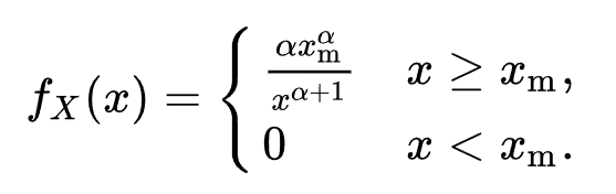
The pdf is only valid when X >= Xm. When Xm = 1, the pdf chart is as follows:

α = tail index. Let’s consider the case where α = 1. In this scenario, the pdf of the Pareto distribution becomes 1/X², so as X increases, the probability exhibits exponential decay. Additionally, in an article from UC Berkeley D-Lab stated that:
….the “80–20 Rule” is represented by a distribution with alpha equal to approximately 1.16.
So, when alpha=1.16, it exhibits the 80/20 rule distribution. As we can see, the consumption distribution in the top right corner of the PowerBI dashboard closely resembles the Pareto distribution. In other words, the majority of people’s consumption is very low, concentrated between $0 to $2 million, while large expenses ($8 million and above) are only affordable by a few individuals. This leads to the aforementioned result: only 30% of people account for 68.43% of total consumption.
Conclusion
This article analyzes 530,000 Black Friday shopping data records using MS SQL, and the findings include:
- Males represent a higher percentage (71.7%) of consumers and also spend more on average, suggesting that males have a stronger purchasing power.
- The top 30% of spenders account for 68.43% of total consumption, indicating a distribution trend closer to the 70/30 rule, rather than the traditional 80/20 rule.
- The group with the highest average spending is ‘male + unmarried + aged 26–35,’ which also constitutes the largest demographic segment at 16%. In contrast, the ‘female + married + aged 55 and above’ group has the lowest average spending.